FLIM Imaging
INTRODUCTION
The following is a short guide to using the new Roper frequency domain FLIM camera installed on the TIRF microscope (room 507) at QBI. Users are strongly encouraged to read the SlideBook 5 FLIM users manual before use. New users are advised to familiarize themselves with frequency domain FLIM and the phasor approach to data analysis before starting. The following papers provide a useful introduction.
1. Polar plot representation of frequency domain FLIM
2. Phasor approach to fluorescence lifetime imaging
STEPS TO ACQUIRING FLIM DATA
1. At least one hour before starting an imaging session, switch on Laserstack, microscope, computer etc power supplies at the wall. Switch on FLIM camera power supply which is located just behind the LaserStack.
2. Switch on Pockels cell high-voltage modulation using box located under desk.
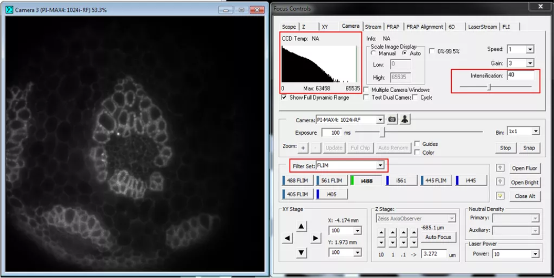
3. Start SlideBook and under “Focus” choose FLIM filter set.
4. Before placing sample on microscope, run the camera live with laser line of choice activated for at least five minutes before starting acquisition. See “Important tips for hardware use” below for explanation.
5. Record calibration. Set exposure time (e.g. 100ms) and adjust intensification under Camera tab until the mean intensity is roughly 2/3 of the dynamic range of the CCD.
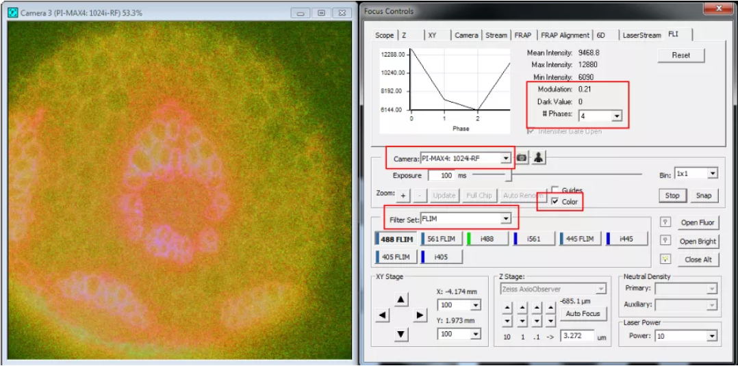
6. With a good signal, select “Color” and inspect “Modulation” parameter under the FLI tab of the focus controls. This parameter should be around 0.2. If this is not the case make an adjustment to the Pockels cell modulation voltage.
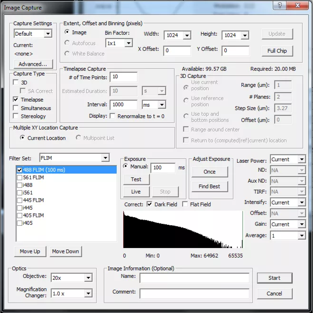
7. In order to calibrate the lifetime record a short timelapse dataset using the “Capture” controls.
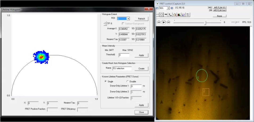
8. Use Image –> Lifetime (FLI) –> Calibrate to enter the known fluorescence lifetime of your calibration sample. Enter the lifetime values in both “Phase lifetime” and “Modulation lifetime”. Click “Compute” and SlideBook will then determine the calibration parameters. Inspect the lifetime data using Image –> Lifetime –> Lifetime Histogram. The reported lifetime should be close to that entered during calibration and all being well the resultant phasor plot should fall on the circle; if it doesn’t see the troubleshooting notes below.
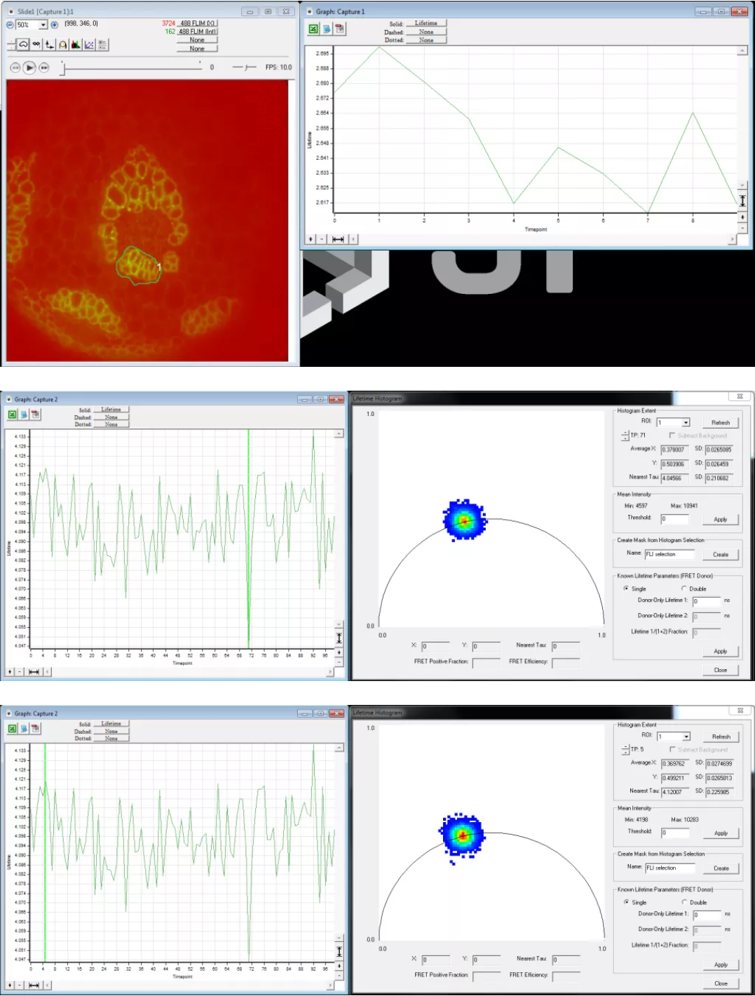
9. Next record sample lifetime. Follow the same procedure as capturing a calibration image. Set exposure time and intensification such that the mean intensity is roughly 2/3 of the CCD dynamic range. If the sample is fixed it is recommended to record a short timelapse sequence to ensure that the lifetime values reported are stable. Frame-to-frame variations in lifetime should be of the order of 80-100ps. See the images below for comparisons of the lifetime histograms where the reported lifetime differs by 60ps. If imaging live samples please be aware of fluctuations in lifetime that result from heating of the Pockel’s cell. See important tips for hardware usage below.
Important tips for hardware use
(i) An element of the laser stack (Pockel’s cell) experiences thermal effects. When the system is first turned on and running the reported sample intensity increases initially and reaches a plateau – it is important to run the system for at least 30 minutes before starting an experiment. Heating in the Pockel’s cell affects the first recorded image and as such data should always be recorded as a time series and the first frame should be disregarded.
(ii) Image-to-image noise is in the 100-200ps range and so repeated measurements are crucial when an attempt is made to measure subtle changes in lifetime in a live cell experiment. Pixel-to-pixel or intra-image noise is low but an appropriate S/N level is required allow the spatial distinction of very subtle changes in lifetime to be detected. It is recommended that that the intensifier is left running for a few minutes before starting any acquisitions. Switch the intensifier gate to open and have the camera running live for at least five minutes before starting the first acquisition.
(ii) The phase of the modulation can change between two states when starting SlideBook. This presents itself by switching the modulation between two states which are 90 degrees out of phase. This means that any calibration performed in one phase state will be invalid in the other. Users should look for the first phase plane to be the highest intensity; if it is not then SlideBook should be restarted until the system is operating in this state.
(iii) The camera format is 1024×1024 pixels. When the coupling with the intensifier is taken into account the resultant format is actually 700×700 (roughly). So, binning the camera 2×2, resulting in a format of 512×512, does not result in a 4x reduction in spatial resolution and will significantly improve S/N. In most circumstances it is advantageous to run the camera in 2×2 binning mode.
(iv) The recommended fluorophores for calibration purposes are HTPS or any variant of Rhodamine. Fluoroscein is not recommended due to the sensitivity of its lifetime to environmental conditions such as pH. When acquiring a calibration data set it is recommended to record a time-lapse series with at least ten frames; inspect the lifetime histogram and discard the first few frames making use of one frame that looks most sensible for the calibration.
(v) The LaserStack now incorporates a 405nm laser. Unfortunately it has been necessary to link the hardware output power control for this laser on the TTL hardware interface to that for the 445nm laser. What this means is that reducing the output power of the 405nm laser on the TTL box also reduces the output power of the 445nm laser. If you reduce the output of the 405nm, remember to return the control to the maximum output when your session has finished so that this does not cause problems for the users of the 445nm laser (e.g. for CFP imaging).
Important Tips for Analysis
Problems such as calibration drift and unstable lifetimes can be attributed to analysis problems. Here are some tips to avoid this:
(i) You must do all lifetime imaging (including calibration) with dark field subtraction checked ON. **both your data and the calibration must be done with this checked. (Unfortunately a bug in SlideBook currently prevents the use of this option, which makes the use of a background very important)
(ii) Use a background. Create a background region in your image before doing any FLIM analysis. The best region is something inside the intensifier area, but outside where there is any signal from the fluor you are looking at. This can even reduce autofluorescence if it is constant in the field. Look at the images I sent you, you will see that adding a background region significantly improves the lifetime measurement and removes the drift from the timelapses. Without this regions of different intensity will seem to have different lifetimes when they shouldn’t.
(iii) Careful calibration. When calibrating with a solution, you often don’t have a signal-less region in the image. So you must use extra care to have good enough signal to noise in the calibration. Any background has a lifetime of infinite, so it can change the calibration quite a bit.
-
- Make sure you are choosing signal more than 10 x the background.
- Instead of calibrating using a large region in the center of the image, use a smaller region in a bright area.
- You can also try making a background region in an area with no signal.
- Lifetime histogram. Use the lifetime histogram for trouble shooting, here is how:
- Data is outside the circle = most likely there was background in your calibration; redo the calibration.
- Data is inside the circle by a lot = Somehow background is in your data or the calibration changed. Redo the calibration and check again. if it is still a problem then you might have some problem with the sample (phenol red does this, or room lights, or bad filters).
- Data is always in the circle when it should be on the circle = there is background in your sample or your calibration. Play with the background region.
- Data has a tail that stretches towards or away from the lower left corner = there is a background problem; move the region.
- Data has a tail that stretches along the circle = this is usually real data. Use regions to find out where exactly the change happens.
- Data forms a huge spot on the circle = low signal to noise. Attempt to set a threshold to remove the presence of low S/N data.
- Data forms a tiny spot, one or three pixels, even though the sample is not super bright = something is wrong, make sure everything is turned on and that you are getting modulation. Maybe you set too high a threshold.

